

The more things change, the more they stay the same. After a week full of economic news, the market ended up almost where it began last week. Will this week break the monotony? Will the popular catchphrase of “sell in May and go away” hold? The media will be using that phrase repeatedly this week.
With the exception of a bit of a wild ride on Monday, the rest of the week was pretty tame with the market probably awaiting the jobs report on Friday. Then the report cemented the lack of commitment of traders at the end of the week, leaving the S&P 500 with about a 1% gain for the entire week.
Monday began with opposing forces tugging at it. Financial stocks were bringing down the house with the surprising news that Bank of America had to cancel its dividend increase and stock buyback plan due to a USD$4 Billion accounting error. On the positive side were the news that pharmaceutical giant Pfizer continued its pursuit of AstraZeneca with a USD$100 billion offer.
The rest of the week was range bound. The US FOMC announced its expected reduction of its asset purchasing program on Wednesday. The first indication of US GDP was a paltry 0.1% versus a 1.1% expectation. Then there was the Friday US monthly jobs report.
The headline number of 288,000 US jobs added versus the 210,000 that were anticipated should have produced at least some reaction in the markets. However, the news was actually somewhat ambiguous. While the total increase in employment was positive, and the unemployment rate decreased, there were some other metrics that give rise to concern. The civilian labor force dropped by 806,000 for the month of April. Arithmetically, this helps bring the unemployment rate down, but signifies that there are 806,000 people who gave up looking for work or retired. The other figure that was scrutinized was the average hourly earnings which was flat from last month but still up 1.9% from a year ago. These factors dampened the effect of the headline number.
It doesn’t require much imagination to see why the headline US employment number has been overlooked recently. A lot more attention has been paid to the other labor statistics released in the report. It has not been easy to tell if the accompanying labor statistics corroborate or contradict perceptions of the strength of the US labor market. For example, in the graph below you will see the labor participation rate of university educated labor participants over the age of 25.
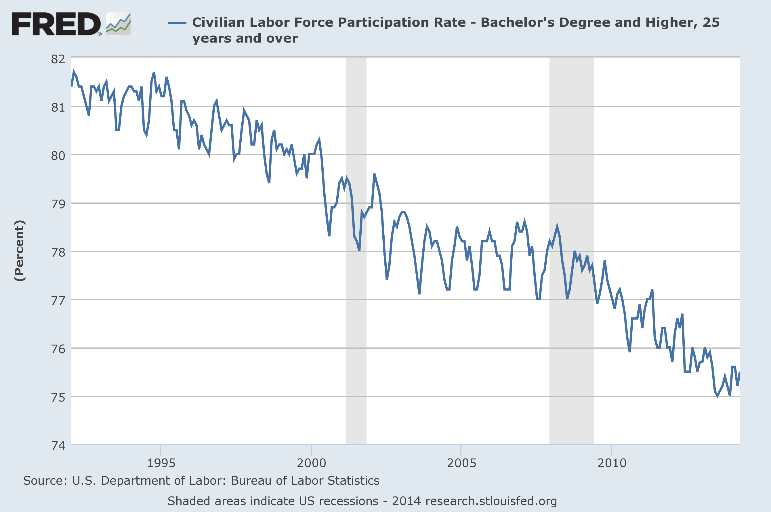 The demographic of persons represented in this graph are those who should be at stages in their careers where they are in a position to earn proportionally larger wage increases. These wages would start them down the path to making large expenditures such as homes, autos, and other large purchases. The decline of this demographic reaching financial stability will have an effect on their purchasing power and on overall consumption in the future. It is this train of thought that has many people concerned with the current state of the US labor market despite positive headline numbers such as in the latest report.
Forget “Sell in May”, it is more appropriate to say “Sell on Friday”. The mixed data of the labor report and increased fears of a flare up in the Ukraine crisis kept things subdued on the last day of the week. In terms of sector performance, there was nothing remarkable to note. It appears that there was some profit taking in some of the recent outperforming sectors such as utilities and oil & gas equipment & services sectors.
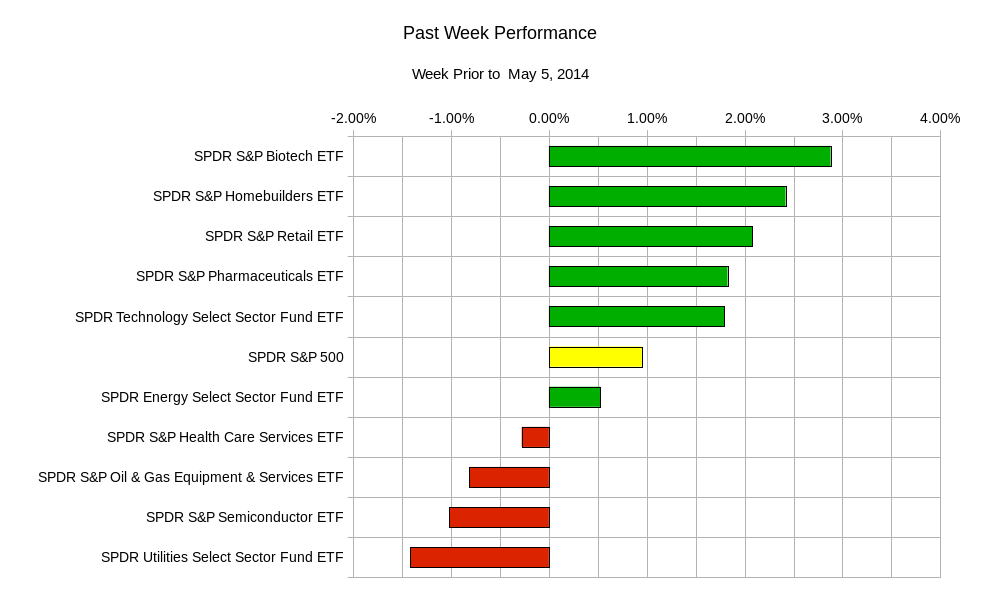 The profit taking helped recent losing sectors such as technology and biotech take a break from the hemorrhaging as of late. Popular momentum names such as Netflix, Google, Priceline, Amazon, and Tesla ended the week in the green.
Is there any merit in the “Sell in May” diatribe? The answer is yes, however it is not as strong an argument as it appears to be. Perhaps it has become more of a tool for the media to have something to talk about when there isn’t much of anything else to talk about. For argument’s sake let us look at how the monthly returns of the S&P 500 index look like for the past 10 years.
| Month | Monthly Return | Rank |
| January | -1.18% | 12 |
| February | -0.78% | 10 |
| March | 3.35% | 1 |
| April | 1.95% | 3 |
| May | -0.84% | 11 |
| June | -0.77% | 8 |
| July | 1.59% | 4 |
| August | -0.77% | 9 |
| September | 0.58% | 6 |
| October | -0.04% | 7 |
| November | 0.60% | 5 |
| December | 3.09% | 2 |
The reasoning behind the idea of “Sell in May” is sound. We see from this table that April ranks as the third best month of the year. This is also after the month of March which tends to be the best performing month of the year. After two months of top performance, you run into May which ranks 11 out of the 12 months, followed by June which is slightly better but still only ranks 8th out of the twelve months. If you bought at any point since January and sold before May you would be profitable.
The likelihood of the “Sell in May” investment thesis being filler for news articles also holds merit. Let us inspect the data from the same past ten years as above. This time we will look at the daily volatility of the S&P 500 index during each month.
| Month | Daily Volatility | Rank |
| January | 1.09% | 9 |
| February | 1.09% | 7 |
| March | 1.27% | 5 |
| April | 0.99% | 12 |
| May | 1.05% | 10 |
| June | 1.09% | 8 |
| July | 0.99% | 11 |
| August | 1.29% | 4 |
| September | 1.40% | 3 |
| October | 1.90% | 1 |
| November | 1.68% | 2 |
| December | 1.20% | 6 |
The data above represents the standard deviation of one day changes in the S&P 500 for each month. This means that for any day during the month of December, about 68% of the time the S&P 500 index will change anywhere from -1.2% to 1.2%. This table tells us that May ranks tenth out of the twelve months in terms of daily volatility. Therefore it is one of the more “quieter” months.
The argument against the idea of “sell in May” is that the groupings of months is somewhat arbitrary. In terms of organization, it is easy to think of investments and trades in the same calendar months that we live in and use for every other aspect of life. However, events, market movements, and your trading can operate in a different time frame. Perhaps if you grouped the market performance in terms of six week groups instead of the twelve months you would get different results. There are no laws that force you to trade in one month time periods that begin and end on the precise begining and end of each month like in the tables above. Nonetheless, it is an interesting set of data to look at and keep in mind.
Returning to a more definitive time frame, here are the upcoming economic and earnings reports for this trading week.
Monday: US ISM non-manufacturing survey, earnings from Pfizer and AIG; Tuesday: Reserve Bank of Australia Interest Rate decision and policy statement Bank of Japan Policy meeting minutes, earnings from Disney, UBS, Electronic Arts, Whole Foods; Wednesday: US Fed Chair Janet Yellen testifies before US Joint Economic Committe, earnings from Tesla, Green Mountain Coffee, A-B InBev; Thursday: Australian Unemployment report, Swiss Consumer Price Index (CPI), Bank of England Interest Rate decision, European Central Bank Rate decision and Policy statement, earnings from Priceline, News Corp, and Nvidia; Friday: Australian Monetary Policy statement and Canadian Unemployment.
The expected landing point for the SPY (S&P 500 ETF) this week is between 183.50 and 191.10. The week could prove to be interesting for commodities with the GLD (Gold ETF) looking to end in between 123.10 and 129.60. The USO (US Oil ETF) may end the week between 35.30 and 37.50.
Regardless of the popularity of different trading strategies or ideas, make sure that the trades and investments that you execute come from a sound and reasonable interpretation of the markets and your tolerance of risk. Just because the rest of the world revolves around a twelve month calendar, does not mean your trading has to.
Good luck and trade rationally.